Triplet example
This triplet design, used in Jose Sasian’s Lens Design OPTI 517 course at the Univ. of Arizona, is attributed to Geiser.
%matplotlib inline
isdark = False
Setup the rayoptics environment
The environment.py module imports many useful classes and functions. All the symbols defined in the module are intended to be imported into a rayoptics interactive session.
from rayoptics.environment import *
Create a new model
Create a new OpticalModel instance and set up some convenient aliases to important constituents of the model.
opm = OpticalModel()
sm  = opm['seq_model']
osp = opm['optical_spec']
pm = opm['parax_model']
em = opm['ele_model']
pt = opm['part_tree']
ar = opm['analysis_results']
Define first order aperture and field for system
The pupil and field specifications can be specified in a variety of
ways. The key keyword argument takes a list of 2 strings. The first
string indicates whether the specification is in object or image space.
The second one indicates which parameter is the defining specification.
The PupilSpec can be defined in object or image space. The defining
parameters can be epd, f/# or NA, where epd is the pupil
diameter.
osp['pupil'] = PupilSpec(osp, key=['object', 'epd'], value=12.5)
The FieldSpec can be defined in object or image space. The defining
parameters can be height or angle, where angle is given in
degrees. The is_relative keyword argument may be used to specify
fields as a fraction of the maximum value
osp['fov'] = FieldSpec(osp, key=['object', 'angle'], value=20.0, flds=[0., 0.707, 1.], is_relative=True)
The WvlSpec defines the wavelengths and weights to use when evaluating the model. The wavelength values can be given in either nanometers or a spectral line designation.
osp['wvls'] = WvlSpec([('F', 0.5), (587.5618, 1.0), ('C', 0.5)], ref_wl=1)
Define interface and gap data for the sequential model
opm.radius_mode = True

sm.gaps[0].thi=1e10

sm.add_surface([23.713, 4.831, 'N-LAK9', 'Schott'])
sm.add_surface([7331.288, 5.86])
sm.add_surface([-24.456, .975, 'N-SF5,Schott'])
sm.set_stop()
sm.add_surface([21.896, 4.822])
sm.add_surface([86.759, 3.127, 'N-LAK9', 'Schott'])
sm.add_surface([-20.4942, 41.2365])
Update the model
opm.update_model()
List the sequential model
sm.list_model()
             r            t        medium     mode   zdr      sd
 Obj:     0.000000  1.00000e+10       air             1  3.6397e+09
   1:    23.713000      4.83100    N-LAK9             1      10.009
   2:  7331.288000      5.86000       air             1      8.9482
Stop:   -24.456000     0.975000     N-SF5             1      4.7919
   4:    21.896000      4.82200       air             1      4.7761
   5:    86.759000      3.12700    N-LAK9             1      8.0217
   6:   -20.494200      41.2365       air             1      8.3321
 Img:     0.000000      0.00000                       1      18.217
List the optical specifications
Use the listobj() function to get formatted output of an object’s contents.
listobj(osp)
aperture: object epd; value=   12.5000
field: object angle; value=   20.0000
y =  0.000 ( 0.00) vlx= 0.000 vux= 0.000 vly= 0.000 vuy= 0.000
y = 14.140 ( 0.71) vlx= 0.000 vux= 0.000 vly= 0.000 vuy= 0.000
y = 20.000 ( 1.00) vlx= 0.000 vux= 0.000 vly= 0.000 vuy= 0.000
is_relative=True, is_wide_angle=False
central wavelength=  587.5618 nm
wavelength (weight) =  486.1327 (0.500),  587.5618 (1.000)*,  656.2725 (0.500)
focus shift=0.0
List the first order properties
pm.first_order_data()
efl                  50
f                    50
f'                   50
ffl               -37.1
pp1                12.9
bfl               41.24
ppk              -8.763
pp sep           -2.047
f/#                   4
m                -5e-09
red              -2e+08
obj_dist          1e+10
obj_ang              20
enp_dist          11.68
enp_radius         6.25
na obj         6.25e-10
n obj                 1
img_dist          41.24
img_ht             18.2
exp_dist         -10.01
exp_radius        6.406
na img           -0.125
n img                 1
optical invariant        2.275
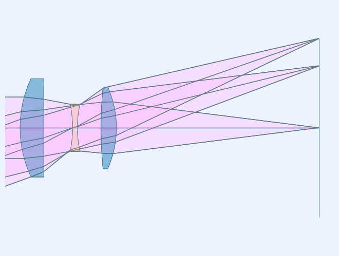
Draw a lens picture
layout_plt = plt.figure(FigureClass=InteractiveLayout, opt_model=opm, is_dark=isdark).plot()
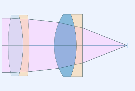
em.list_model()
0: Object (DummyInterface): Surface(lbl='Obj', profile=Spherical(c=0.0), interact_mode='dummy')
1: E1 (Element): Element: Spherical(c=0.042170961076202926), Spherical(c=0.00013640168003221264), t=4.8310, sd=10.0087, glass: N-LAK9
2: E2 (Element): Element: Spherical(c=-0.04088976120379457), Spherical(c=0.04567044208987943), t=0.9750, sd=4.7919, glass: N-SF5
3: E3 (Element): Element: Spherical(c=0.011526181721781025), Spherical(c=-0.04879429301948844), t=3.1270, sd=8.3321, glass: N-LAK9
4: Image (DummyInterface): Surface(lbl='Img', profile=Spherical(c=0.0), interact_mode='dummy')
pm.list_model()
          ax_ht        pr_ht       ax_slp       pr_slp         power          tau        index    type
0:            0  -3.6397e+09     6.25e-10      0.36397             0        1e+10      1.00000    dummy
1:         6.25     -4.25088    -0.182126     0.487842    0.02914022      2.85689      1.69100    transmit
2:      5.72969     -2.85718    -0.181586     0.487573 -9.425384e-05         5.86      1.00000    transmit
3:      4.66559  3.53405e-07   -0.0532508     0.487573   -0.02750683     0.582887      1.67271    transmit
4:      4.63455       0.2842    0.0891357     0.496304   -0.03072283        4.822      1.00000    transmit
5:      5.06436      2.67738       0.0488      0.47498   0.007964615       1.8492      1.69100    transmit
6:       5.1546      3.55571    -0.124998     0.355092    0.03371696      41.2365      1.00000    transmit
7:  0.000143648      18.1985    -0.124998     0.355092             0            0      1.00000    dummy
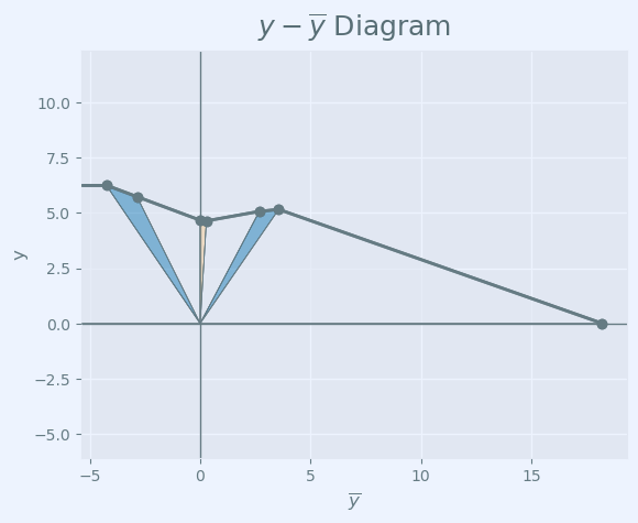
Draw a \(y-\overline{y}\) diagram
yybar_plt = plt.figure(FigureClass=InteractiveDiagram, opt_model=opm, dgm_type='ht',
                       do_draw_axes=True, do_draw_frame=True, is_dark=isdark).plot()
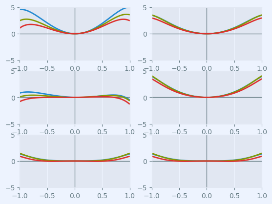
Plot the transverse ray aberrations
abr_plt = plt.figure(FigureClass=RayFanFigure, opt_model=opm, data_type='Ray', scale_type=Fit.All_Same, is_dark=isdark).plot()
Plot the wavefront aberration
wav_plt = plt.figure(FigureClass=RayFanFigure, opt_model=opm, data_type='OPD', scale_type=Fit.All_Same, is_dark=isdark).plot()
List the paraxial model
pm.list_model()
          ax_ht        pr_ht       ax_slp       pr_slp         power          tau        index    type
0:            0  -3.6397e+09     6.25e-10      0.36397             0        1e+10      1.00000    dummy
1:         6.25     -4.25088    -0.182126     0.487842    0.02914022      2.85689      1.69100    transmit
2:      5.72969     -2.85718    -0.181586     0.487573 -9.425384e-05         5.86      1.00000    transmit
3:      4.66559  3.53405e-07   -0.0532508     0.487573   -0.02750683     0.582887      1.67271    transmit
4:      4.63455       0.2842    0.0891357     0.496304   -0.03072283        4.822      1.00000    transmit
5:      5.06436      2.67738       0.0488      0.47498   0.007964615       1.8492      1.69100    transmit
6:       5.1546      3.55571    -0.124998     0.355092    0.03371696      41.2365      1.00000    transmit
7:  0.000143648      18.1985    -0.124998     0.355092             0            0      1.00000    dummy
pm.list_lens()
      ax_ray_ht    ax_ray_slp
0:            0      6.25e-10
1:         6.25     -0.182126
2:      5.72969     -0.181586
3:      4.66559    -0.0532508
4:      4.63455     0.0891357
5:      5.06436        0.0488
6:       5.1546     -0.124998
7:  0.000143648     -0.124998

      pr_ray_ht    pr_ray_slp
0:  -3.6397e+09       0.36397
1:     -4.25088      0.487842
2:     -2.85718      0.487573
3:  3.53405e-07      0.487573
4:       0.2842      0.496304
5:      2.67738       0.47498
6:      3.55571      0.355092
7:      18.1985      0.355092

           power           tau        index    type
0:             0         1e+10      1.00000    dummy
1:    0.02914022        2.8569      1.69100    transmit
2: -9.425384e-05          5.86      1.00000    transmit
3:   -0.02750683       0.58289      1.67271    transmit
4:   -0.03072283         4.822      1.00000    transmit
5:   0.007964615        1.8492      1.69100    transmit
6:    0.03371696        41.236      1.00000    transmit
7:             0             0      1.00000    dummy
Third Order Seidel aberrations
Computation and tabular display
to_pkg = compute_third_order(opm)
to_pkg
| S-I | S-II | S-III | S-IV | S-V | |
|---|---|---|---|---|---|
| 1 | 0.027654 | 0.019379 | 0.013581 | 0.089174 | 0.072010 |
| 2 | 0.022082 | -0.059501 | 0.160327 | -0.000288 | -0.431229 |
| 3 | -0.105156 | 0.137692 | -0.180295 | -0.085097 | 0.347506 |
| 4 | -0.045358 | -0.076796 | -0.130024 | -0.095046 | -0.381069 |
| 5 | 0.007942 | 0.028382 | 0.101431 | 0.024373 | 0.449596 |
| 6 | 0.103810 | -0.050068 | 0.024148 | 0.103180 | -0.061411 |
| sum | 0.010973 | -0.000912 | -0.010832 | 0.036297 | -0.004597 |
Bar chart for surface by surface third order aberrations
fig, ax = plt.subplots()
ax.set_xlabel('Surface')
ax.set_ylabel('third order aberration')
ax.set_title('Surface by surface third order aberrations')
to_pkg.plot.bar(ax=ax, rot=0)
ax.grid(True)
fig.tight_layout()

convert aberration sums to transverse measure
ax_ray, pr_ray, fod = ar['parax_data']
n_last = pm.sys[-1][mc.indx]
u_last = ax_ray[-1][mc.slp]
to.seidel_to_transverse_aberration(to_pkg.loc['sum',:], n_last, u_last)
TSA   -0.043893
TCO    0.010944
TAS   -0.015198
SAS   -0.101860
PTB   -0.145190
DST    0.018387
dtype: float64
convert sums to wavefront measure
central_wv = opm.nm_to_sys_units(sm.central_wavelength())
to.seidel_to_wavefront(to_pkg.loc['sum',:], central_wv).T
W040     2.334457
W131    -0.776108
W222    -9.218154
W220    10.834770
W311    -3.911650
dtype: float64
compute Petzval, sagittal and tangential field curvature
to.seidel_to_field_curv(to_pkg.loc['sum',:], n_last, fod.opt_inv)
TCV    0.000734
SCV    0.004921
PCV    0.007014
dtype: float64
Save the model
opm.save_model('Sasian Triplet')