Multiple lens import example
This notebook shows the steps to follow to open multiple vendor component files using ray-optics.
%matplotlib inline
# initialization
from rayoptics.environment import *
root_pth = Path(rayoptics.__file__).resolve().parent
Create a new, empty, Optical Model
opm = OpticalModel()
sm = opm['seq_model']
osp = opm['optical_spec']
pm = opm['parax_model']
em = opm['ele_model']
pt = opm['part_tree']
By default, the sequential model will automatically recalculate lens apertures when the model changes. The imported lenses will have apertures defined, so turn the do_apertures setting off.
sm.do_apertures = False
Set the object distance of the empty Optical Model to infinity (1e10 is close enough).
sm.gaps[0].thi = 1e10
Listing the sequential model shows object and image interfaces and the air-filled object distance gap.
sm.list_model()
            c            t        medium     mode   zdr      sd
Obj:     0.000000  1.00000e+10       air             1      1.0000
Img:     0.000000      0.00000                       1      1.0000
Enter the Optical Specifications
The usage specifications for the optical system are defined via different properties of the OpticalSpecs class.
osp.pupil.value=22
listobj(osp['pupil'])
aperture: object epd; value=22
opm.update_model()
Add first component
The parameter t is the spacing following the inserted component.
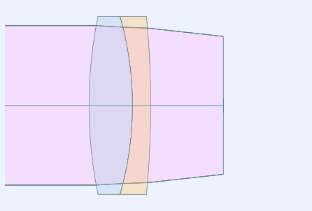
opm.add_from_file(root_pth/"codev/tests/CODV_32327.seq", t=10.)
The listing shows the imported part is a cemented lens doublet.
sm.list_model()
              c            t        medium     mode   zdr      sd
  Obj:     0.000000  1.00000e+10       air             1      1.0000
32327:     0.016268      6.00000     N-BK7             1      12.000
    2:    -0.022401      2.50000     N-SF5             1      1.0000
    3:    -0.007696      10.0000       air             1      12.000
  Img:     0.000000      0.00000                       1      1.0000
The part tree can be displayed using list_model on the part_tree.
pt.list_model()
root
├── Object
├── CE1
└── Image
Generate a lens picture
This is done using the interactivelayout module.
All graphics in rayoptics are based on matplotlib.
layout_plt = plt.figure(FigureClass=InteractiveLayout, opt_model=opm,
                        do_draw_rays=True, do_paraxial_layout=False).plot()
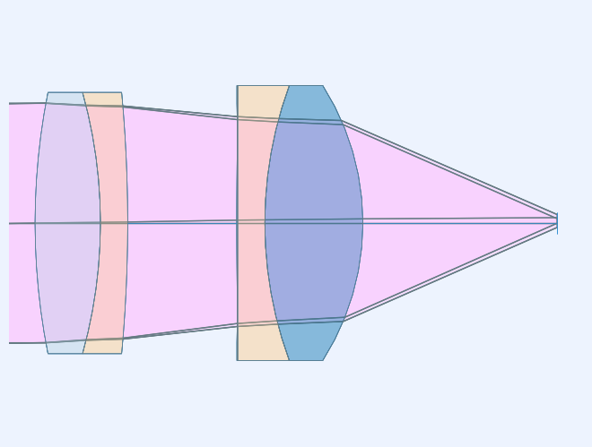
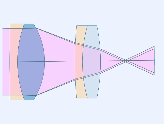
Add the second component
opm.add_from_file(root_pth/"codev/tests/CODV_49664.seq", t=17.8)
The imported element, CE2, is a triplet with a thin, aspheric, cap.
sm.list_model()
              c            t        medium     mode   zdr      sd
  Obj:     0.000000  1.00000e+10       air             1      1.0000
32327:     0.016268      6.00000     N-BK7             1      12.000
    2:    -0.022401      2.50000     N-SF5             1      1.0000
    3:    -0.007696      10.0000       air             1      12.000
49663:     0.042553      9.00000   S-LAL 8             1      12.629
    5:    -0.027248      2.50000   S-TIH53             1      11.842
    6:     0.000000    0.0800000 517000.520000             1      11.004
    7:    -0.003096      17.8000       air             1      10.990
  Img:     0.000000      0.00000                       1      1.0000
opm.update_model()
Use the listobj() function to get formatted output of an object’s contents.
listobj(sm.ifcs[7].profile)
profile: EvenPolynomial
c=-0.003095913950326,   r=-323.006393602994   conic cnst=0.0
coefficients: [0.0, 1.38925111836e-05, -2.08175206307e-08, 0.0, 0.0, 0.0, 0.0, 0.0, 0.0, 0.0]
pt.list_model()
root
├── Object
├── CE1
├── CE2
└── Image
em.list_model()
0: Object (DummyInterface): Surface(lbl='Obj', profile=Spherical(c=0.0), interact_mode='dummy')
1: CE1 (CementedElement): CementedElement: [1, 2, 3]
2: CE2 (CementedElement): CementedElement: [4, 5, 6, 7]
3: Image (DummyInterface): Surface(lbl='Img', profile=Spherical(c=0.0), interact_mode='dummy')
layout_plt0 = plt.figure(FigureClass=InteractiveLayout, opt_model=opm,
                        do_draw_rays=True, do_paraxial_layout=False).plot()
Flipping a lens element
It is common that importing components in this fashion the the catalog ordering of the surfaces is not what a particular optical model needs. The flip() can be used to flip elements and/or sequences of interfaces.
First, retrieve the element definitions from the part tree.
ce1 = pt.obj_by_name('CE1')
ce2 = pt.obj_by_name('CE2')
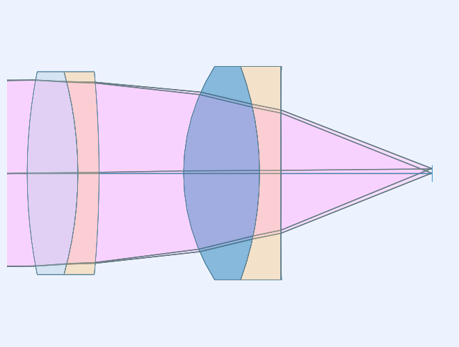
Flip the second cemented element.
opm.flip(ce2)
layout_plt1 = plt.figure(FigureClass=InteractiveLayout, opt_model=opm,
                        do_draw_rays=True, do_paraxial_layout=False).plot()
Restore the element to its original orientation.
opm.flip(ce2)
layout_plt2 = plt.figure(FigureClass=InteractiveLayout, opt_model=opm,
                        do_draw_rays=True, do_paraxial_layout=False).plot()
Flip operation for a range of Interfaces
Sometimes it is more convenient to specify a range of interface indices.
sm.list_model()
              c            t        medium     mode   zdr      sd
  Obj:     0.000000  1.00000e+10       air             1      1.0000
32327:     0.016268      6.00000     N-BK7             1      12.000
    2:    -0.022401      2.50000     N-SF5             1      1.0000
    3:    -0.007696      10.0000       air             1      12.000
49663:     0.042553      9.00000   S-LAL 8             1      12.629
    5:    -0.027248      2.50000   S-TIH53             1      11.842
    6:     0.000000    0.0800000 517000.520000             1      11.004
    7:    -0.003096      17.8000       air             1      10.990
  Img:     0.000000      0.00000                       1      1.0000
If we want to flip the lens assembly end for end, we would want to flip the range of interfaces from 1 to 7.
opm.flip(1,7)
sm.list_model()
              c            t        medium     mode   zdr      sd
  Obj:     0.000000  1.00000e+10       air             1      1.0000
    1:     0.003096    0.0800000 517000.520000             1      10.990
    2:    -0.000000      2.50000   S-TIH53             1      11.004
    3:     0.027248      9.00000   S-LAL 8             1      11.842
49663:    -0.042553      10.0000       air             1      12.629
    5:     0.007696      2.50000     N-SF5             1      12.000
    6:     0.022401      6.00000     N-BK7             1      1.0000
32327:    -0.016268      17.8000       air             1      12.000
  Img:     0.000000      0.00000                       1      1.0000
layout_plt3 = plt.figure(FigureClass=InteractiveLayout, opt_model=opm,
                        do_draw_rays=True, do_paraxial_layout=False).plot()
All of the information is transformed by the flip() operation; this can be seen be using listobj() on the 1st interface of the sequential model.
listobj(sm.ifcs[1])
transmit
profile: EvenPolynomial
c=0.003095913950326,   r=323.006393602994   conic cnst=0.0
coefficients: [-0.0, -1.38925111836e-05, 2.08175206307e-08, -0.0, -0.0, -0.0, -0.0, -0.0, -0.0, -0.0]
surface_od=10.990183852239241