Edmund catalog lens example
This notebook shows the steps to follow to open a CODE V seq file of a Edmund achromatic doublet.
%matplotlib inline
# initialization
from rayoptics.environment import *
Use the object oriented filesystem interface from Python 3
root_pth = Path(rayoptics.__file__).resolve().parent
Read CODE V seq file for Edmund part 32-327, Achromatic Lens
Use the open_model() function to read CODE V .seq files, Zemax .zmx files, and the native rayoptics JSON files, .roa
It returns an instance of OpticalModel that contains all of the model data.
opm = open_model(root_pth/"codev/tests/CODV_32327.seq")
Setup convenient aliases for using rayoptics functions
sm  = opm['seq_model']
osp = opm['optical_spec']
pm = opm['parax_model']
em = opm['ele_model']
pt = opm['part_tree']
ar = opm['analysis_results']
sm.list_model()
              r            t        medium     mode   zdr      sd
  Obj:     0.000000  1.00000e+13       air             1      1.0000
32327:    61.470000      6.00000     N-BK7             1      12.000
    2:   -44.640000      2.50000     N-SF5             1      1.0000
    3:  -129.940000      95.9519       air             1      12.000
  Img:     0.000000      0.00000                       1      1.0000
sm.list_sg()
               r               mode              type          y       alpha
                       t           medium
  Obj:      0.00000
                 1.00000e+13          air
32327:      61.4700
                     6.00000        N-BK7
    2:     -44.6400
                     2.50000        N-SF5
    3:     -129.940
                     95.9519          air
  Img:      0.00000
Display first order properties of the model
The calculated first order data is in the FirstOrderData class.
An instance of FirstOrderData is maintained in OpticalModel[‘analysis_results’] under the key parax_data.
Other essential optical specification data is also managed by the OpticalSpecs class:
spectral_region (
WvlSpec)pupil (
PupilSpec)field_of_view (
FieldSpec)defocus (
FocusRange)
A convenience method in ParaxialModel, first_order_data(), can be used to display the first order properties of the model.
pm.first_order_data()
efl                 100
f                   100
f'                  100
ffl              -98.58
pp1               1.451
bfl               95.95
ppk              -4.079
pp sep             2.97
f/#               4.001
m                -1e-11
red          -9.997e+10
obj_dist          1e+13
obj_ang               1
enp_dist             -0
enp_radius         12.5
na obj         1.25e-12
n obj                 1
img_dist          95.95
img_ht            1.746
exp_dist         -5.551
exp_radius        12.68
na img           -0.124
n img                 1
optical invariant       0.2182
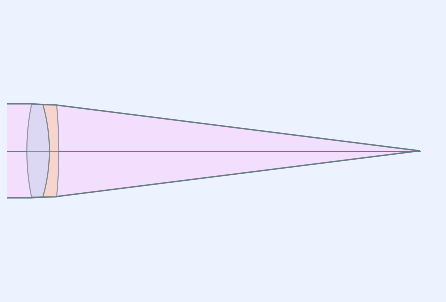
Generate a lens picture
This is done using the interactivelayout module.
All graphics in rayoptics are based on matplotlib.
layout_plt = plt.figure(FigureClass=InteractiveLayout, opt_model=opm,
                        do_draw_rays=True, do_paraxial_layout=False).plot()
Draw a transverse ray aberration plot
This is done using the axisarrayfigure module.
abr_plt = plt.figure(FigureClass=RayFanFigure, opt_model=opm, data_type='Ray',
                     scale_type=Fit.All_Same).plot()
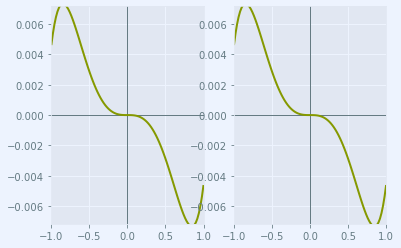
The model in the CODE V seq file only had 1 wavelength defined. Use the OpticalSpecs instance, osp, to modify the spectral_region in the optical subpackage to add wavelengths in the red and blue. The wavelenghts can be specified directly in nm or by using spectral line designations, as done here.
osp['wvls'].set_from_list([['F', 1], ['d', 2], ['C', 1]])
osp['wvls'].reference_wvl = 1
osp['wvls'].wavelengths
[486.1327, 587.5618, 656.2725]
After changing the wavelengths, update the optical model using update_model() to ensure all of the data is consistent.
The OpticalModel class is in the opticalmodel module in the optical subpackage.
opm.update_model()
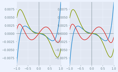
The aberration plot can be updated by calling refresh() on abr_plt
abr_plt.refresh()