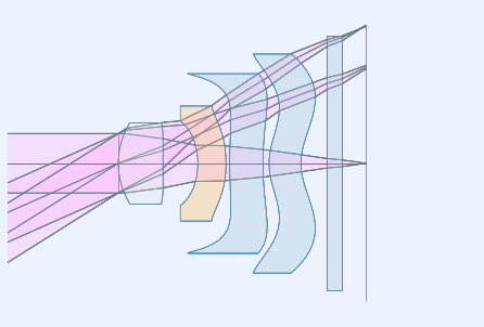
Cell Phone Camera Lens
From U.S. Patent 7,535,658
%matplotlib inline
isdark = False
# use standard rayoptics environment
from rayoptics.environment import *

# util functions
from rayoptics.util.misc_math import normalize
Create a new, empty, model
opm = OpticalModel()
sm = opm['seq_model']
osp = opm['optical_spec']
pm = opm['parax_model']
em = opm['ele_model']
pt = opm['part_tree']
Specify aperture, field, and wavelengths
osp['pupil'] = PupilSpec(osp, key=['image', 'f/#'], value=3.5)
osp['fov'] = FieldSpec(osp, key=['image', 'height'], value=3.5, is_relative=True, flds=[0., .7071, 1])
osp['wvls'] = WvlSpec([('F', 0.5), ('d', 1.0), ('C', 0.5)], ref_wl=1)
Define interface and gap data for the sequential model
The add_surface() method is used to enter a sequential model in the form it’s usually given:
curvature/radius, thickness, glass/refractive index, clear aperture
Each Surface has a profile attribute that is initialized to Spherical.
The profiles module has a variety of non-spherical profiles. Create an instance of the desired profile type and assign it to the profile attribute of the current interface.
opm.radius_mode = True

sm.gaps[0].thi=1e10

sm.add_surface([0., 0.])
sm.set_stop()

sm.add_surface([1.962, 1.19, 1.471, 76.6])
sm.ifcs[sm.cur_surface].profile = RadialPolynomial(r=1.962, ec=2.153,
                        coefs=[0., 0., -1.895e-2, 2.426e-2, -5.123e-2, 8.371e-4, 7.850e-3, 4.091e-3, -7.732e-3, -4.265e-3])

sm.add_surface([33.398, .93])
sm.ifcs[sm.cur_surface].profile = RadialPolynomial(r=33.398, ec=40.18,
                        coefs=[0., 0., -4.966e-3, -1.434e-2, -6.139e-3, -9.284e-5, 6.438e-3, -5.72e-3, -2.385e-2, 1.108e-2])

sm.add_surface([-2.182, .75, 1.603, 27.5])
sm.ifcs[sm.cur_surface].profile = RadialPolynomial(r=-2.182, ec=2.105,
                        coefs=[0., 0., -4.388e-2, -2.555e-2, 5.16e-2, -4.307e-2, -2.831e-2, 3.162e-2, 4.630e-2, -4.877e-2])

sm.add_surface([-6.367, 0.1])
sm.ifcs[sm.cur_surface].profile = RadialPolynomial(r=-6.367, ec=3.382,
                        coefs=[0., 0., -1.131e-1, -7.863e-2, 1.094e-1, 6.228e-3, -2.216e-2, -5.89e-3, 4.123e-3, 1.041e-3])

sm.add_surface([5.694, .89, 1.510, 56.2])
sm.ifcs[sm.cur_surface].profile = RadialPolynomial(r=5.694, ec=-221.1,
                        coefs=[0., 0., -7.876e-2, 7.02e-2, 1.575e-3, -9.958e-3, -7.322e-3, 6.914e-4, 2.54e-3, -7.65e-4])

sm.add_surface([9.192, .16])
sm.ifcs[sm.cur_surface].profile = RadialPolynomial(r=9.192, ec=0.9331,
                        coefs=[0., 0., 9.694e-3, -2.516e-3, -3.606e-3, -2.497e-4, -6.84e-4, -1.414e-4, 2.932e-4, -7.284e-5])

sm.add_surface([1.674, .85, 1.510, 56.2])
sm.ifcs[sm.cur_surface].profile = RadialPolynomial(r=1.674, ec=-7.617,
                        coefs=[0., 0., 7.429e-2, -6.933e-2, -5.811e-3, 2.396e-3, 2.100e-3, -3.119e-4, -5.552e-5, 7.969e-6])

sm.add_surface([1.509, .70])
sm.ifcs[sm.cur_surface].profile = RadialPolynomial(r=1.509, ec=-2.707,
                        coefs=[0., 0., 1.767e-3, -4.652e-2, 1.625e-2, -3.522e-3, -7.106e-4, 3.825e-4, 6.271e-5, -2.631e-5])

sm.add_surface([0., .40, 1.516, 64.1])
sm.add_surface([0., .64])
Update the model
opm.update_model()
Turn off automatically resizing apertures based on sequential model ray trace.
sm.do_apertures = False
List the sequential model and the first order properties
sm.list_model()
             r            t        medium     mode   zdr      sd
 Obj:     0.000000  1.00000e+10       air             1  6.1915e+09
Stop:     0.000000      0.00000       air             1     0.79358
   2:     1.962000      1.19000   471.766             1     0.93439
   3:    33.398000     0.930000       air             1      1.0782
   4:    -2.182000     0.750000   603.275             1      1.1289
   5:    -6.367000     0.100000       air             1      1.5270
   6:     5.694000     0.890000   510.562             1      1.8048
   7:     9.192000     0.160000       air             1      2.3576
   8:     1.674000     0.850000   510.562             1      2.4382
   9:     1.509000     0.700000       air             1      2.8879
  10:     0.000000     0.400000   516.641             1      3.2480
  11:     0.000000     0.640000       air             1      3.3477
 Img:     0.000000      0.00000                       1      3.6298
pm.first_order_data()
efl               5.555
f                 5.555
f'                5.555
ffl              -7.531
pp1              -1.976
bfl              0.5678
ppk              -4.987
pp sep            2.959
f/#                 3.5
m            -5.555e-10
red            -1.8e+09
obj_dist          1e+10
obj_ang           31.76
enp_dist             -0
enp_radius       0.7936
na obj        7.936e-11
n obj                 1
img_dist         0.5678
img_ht            3.439
exp_dist         -3.602
exp_radius       0.5854
na img          -0.1429
n img                 1
optical invariant       0.4913
pt.list_model()
root
├── Object
├── S1
├── E1
├── E2
├── E3
├── E4
├── E5
└── Image
layout_plt0 = plt.figure(FigureClass=InteractiveLayout, opt_model=opm,
                        do_draw_rays=True, do_paraxial_layout=False,
                        is_dark=isdark).plot()
Set semi-diameters and flats for manufacturing and mounting
Note that in the lens layout above, the very aspheric surface shapes lead to extreme lens element shapes. The default logic used by ray-optics to apply flat bevels to concave surfaces is defeated by the aspherics that switch concavity between vertex and edge. How ray-optics renders flats can be controlled on a surface by surface basis.
First, retrieve the lens elements from the part tree.
e1 = pt.obj_by_name('E1')
e2 = pt.obj_by_name('E2')
e3 = pt.obj_by_name('E3')
e4 = pt.obj_by_name('E4')
e5 = pt.obj_by_name('E5')
Lens elements have two surfaces, each of which can be specified with or without a flat.
e2.do_flat1 = 'always'
e2.do_flat2 = 'always'
e3.do_flat1 = 'always'
e3.do_flat2 = 'always'
e4.do_flat1 = 'always'
e4.do_flat2 = 'always'
layout_plt1 = plt.figure(FigureClass=InteractiveLayout, opt_model=opm,
                        do_draw_rays=True, do_paraxial_layout=False,
                        is_dark=isdark).plot()
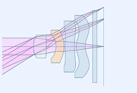
By default, the inside diameters of a flat are set to the clear aperture of the interface in the sequential model. This can be overriden for each surface. The semi-diameter sd() of the lens element may also be set explicitly.
e1.sd = 1.25

e2.sd = 1.75
e2.flat1 = 1.25
e2.flat2 = 1.645

e3.sd = 2.5
e3.flat1 = 2.1

e4.sd = 3.0
e4.flat1 = 2.6

e5.sd = 3.5
Draw a lens layout to verify the model
layout_plt = plt.figure(FigureClass=InteractiveLayout, opt_model=opm,
                        do_draw_rays=True, do_paraxial_layout=False,
                        is_dark=isdark).plot()

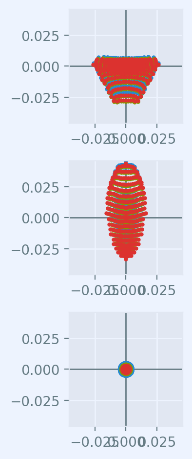
Plot a Spot Diagram
spot_plt = plt.figure(FigureClass=SpotDiagramFigure, opt_model=opm,
                      scale_type=Fit.All_Same, dpi=200, is_dark=isdark).plot()
Save the model
opm.save_model("cell_phone_camera")
Trace axial marginal ray
pt0 = np.array([0., 1., 0.])
dir0 = np.array([0., 0., 1.])
wvl = sm.central_wavelength()
marg_ray = rt.trace(sm, pt0, dir0, wvl)
list_ray(marg_ray[0])
           X            Y            Z           L            M            N               Len
 0:      0.00000      1.00000            0     0.000000     0.000000     1.000000        1e+10
 1:      0.00000      1.00000            0     0.000000     0.000000     1.000000      0.26119
 2:      0.00000      1.00000      0.26119     0.000000    -0.163284     0.986579      0.93632
 3:      0.00000      0.84711   -0.0050525     0.000000    -0.272278     0.962219      0.86687
 4:      0.00000      0.61108     -0.10094     0.000000    -0.024063     0.999710      0.79796
 5:      0.00000      0.59188    -0.053212     0.000000    -0.171810     0.985130      0.16841
 6:      0.00000      0.56295     0.012694     0.000000    -0.122925     0.992416      0.89598
 7:      0.00000      0.45281      0.01188     0.000000    -0.158261     0.987397       0.2017
 8:      0.00000      0.42089     0.051033     0.000000    -0.178956     0.983857      0.83614
 9:      0.00000      0.27126     0.023675     0.000000    -0.185004     0.982738       0.6882
10:      0.00000      0.14394            0     0.000000    -0.122034     0.992526      0.40301
11:      0.00000      0.09476            0     0.000000    -0.185004     0.982738      0.65124
12:      0.00000     -0.02573            0     0.000000    -0.185004     0.982738            0
Trace an arbitrary skew ray
Given a point and direction at the first (not object) interface
dir0 = normalize(np.array([0.086, 0.173, 0.981]))
pt1 = np.array(-dir0)
sm.gaps[1].thi = dir0[2]
pt1[2] = 0.
dir0, [0.086, 0.173, 0.981], pt1
(array([0.08601351, 0.17302717, 0.98115405]),
 [0.086, 0.173, 0.981],
 array([-0.08601351, -0.17302717,  0.        ]))
Use the low level trace_raw() function to trace the ray.
wvl = sm.central_wavelength()

path = sm.path(wl=wvl, start=1)
skew_ray = rt.trace_raw(path, pt1, dir0, wvl)

list_ray(skew_ray[0])
           X            Y            Z           L            M            N               Len
 0:     -0.08601     -0.17303            0     0.086014     0.173027     0.981154     0.009449
 1:     -0.08520     -0.17139     0.009271     0.072254     0.145349     0.986739       1.1966
 2:      0.00126      0.00253   1.1955e-07     0.106304     0.213844     0.971066      0.94474
 3:      0.10169      0.20456    -0.012595     0.085295     0.171581     0.981471      0.75899
 4:      0.16643      0.33479    -0.017664     0.106581     0.214401     0.970913      0.12979
 5:      0.18026      0.36261    0.0083478     0.066253     0.133277     0.988862      0.90879
 6:      0.24047      0.48374     0.017019     0.115071     0.231480     0.966010      0.24881
 7:      0.26910      0.54133     0.097372     0.032613     0.065605     0.997313      0.88059
 8:      0.29782      0.59910       0.1256     0.126731     0.254936     0.958617       0.5992
 9:      0.37376      0.75186            0     0.083596     0.168164     0.982208      0.40725
10:      0.40780      0.82034            0     0.126731     0.254936     0.958617      0.66763
11:      0.49241      0.99054            0     0.126731     0.254936     0.958617            0
Set up the ray trace for the second field point
(field point index = 1)
fld, wvl, foc = osp.lookup_fld_wvl_focus(1)
Trace central, upper and lower rays
Use the trace_ray() function to trace a ray in terms of pupil position, field point and wavelength.
ray_f1_r0 = trace_ray(opm, [0., 0.], fld, wvl)
list_ray(ray_f1_r0)
           X            Y            Z           L            M            N               Len
 0:      0.00000 -4133992479.29825            0     0.000000     0.382041     0.924145   1.0821e+10
 1:      0.00000     -0.00000            0     0.000000     0.382041     0.924145   2.6785e-14
 2:      0.00000     -0.00000   2.4226e-14     0.000000     0.259715     0.965685       1.2335
 3:      0.00000      0.32037    0.0012037     0.000000     0.384968     0.922930      0.87739
 4:      0.00000      0.65813     -0.11903     0.000000     0.381160     0.924509      0.76657
 5:      0.00000      0.95032     -0.16032     0.000000     0.400332     0.916370      0.31265
 6:      0.00000      1.07549     0.026181     0.000000     0.257929     0.966164       0.9887
 7:      0.00000      1.33050     0.091422     0.000000     0.441538     0.897243       0.3836
 8:      0.00000      1.49987      0.27561     0.000000     0.300087     0.953912       1.0019
 9:      0.00000      1.80052      0.38131     0.000000     0.428907     0.903348      0.35279
10:      0.00000      1.95184            0     0.000000     0.282920     0.959143      0.41704
11:      0.00000      2.06983            0     0.000000     0.428907     0.903348      0.70848
12:      0.00000      2.37370            0     0.000000     0.428907     0.903348            0
ray_f1_py = trace_ray(opm, [0., 1.], fld, wvl)
list_ray(ray_f1_py)
           X            Y            Z           L            M            N               Len
 0:      0.00000 -4133992479.29825            0     0.000000     0.382041     0.924145   1.0821e+10
 1:      0.00000      0.79358            0     0.000000     0.382041     0.924145      0.21569
 2:      0.00000      0.87598      0.19933     0.000000     0.088675     0.996061      0.97797
 3:      0.00000      0.96270    -0.016556     0.000000     0.064387     0.997925        0.623
 4:      0.00000      1.00282     -0.32485     0.000000     0.322392     0.946606      0.82812
 5:      0.00000      1.26980     -0.29095     0.000000     0.281957     0.959427      0.43129
 6:      0.00000      1.39140     0.022842     0.000000     0.208223     0.978081      0.99819
 7:      0.00000      1.59925      0.10915     0.000000     0.329759     0.944065      0.32274
 8:      0.00000      1.70567      0.25384     0.000000     0.283035     0.959110      0.99581
 9:      0.00000      1.98752      0.35893     0.000000     0.328025     0.944669      0.36105
10:      0.00000      2.10595            0     0.000000     0.216375     0.976310      0.40971
11:      0.00000      2.19460            0     0.000000     0.328025     0.944669      0.67749
12:      0.00000      2.41684            0     0.000000     0.328025     0.944669            0
ray_f1_my = trace_ray(opm, [0., -1.], fld, wvl)
list_ray(ray_f1_my)
           X            Y            Z           L            M            N               Len
 0:      0.00000 -4133992479.29825            0     0.000000     0.382041     0.924145   1.0821e+10
 1:      0.00000     -0.79358            0     0.000000     0.382041     0.924145      0.15109
 2:      0.00000     -0.73586      0.13963     0.000000     0.375277     0.926913       1.1344
 3:      0.00000     -0.31014    0.0011435     0.000000     0.548928     0.835870       1.0872
 4:      0.00000      0.28664    -0.020134     0.000000     0.400058     0.916490      0.78058
 5:      0.00000      0.59891    -0.054742     0.000000     0.508026     0.861342      0.19864
 6:      0.00000      0.69983     0.016354     0.000000     0.326388     0.945236       0.9873
 7:      0.00000      1.02207     0.059586     0.000000     0.555786     0.831326      0.43431
 8:      0.00000      1.26345      0.26064     0.000000     0.312257     0.949998        1.014
 9:      0.00000      1.58007       0.3739     0.000000     0.534422     0.845218      0.38582
10:      0.00000      1.78626            0     0.000000     0.352521     0.935804      0.42744
11:      0.00000      1.93694            0     0.000000     0.534422     0.845218       0.7572
12:      0.00000      2.34160            0     0.000000     0.534422     0.845218            0